2D Shock Wave/Laminar Boundary-Layer Interaction

Problem Description

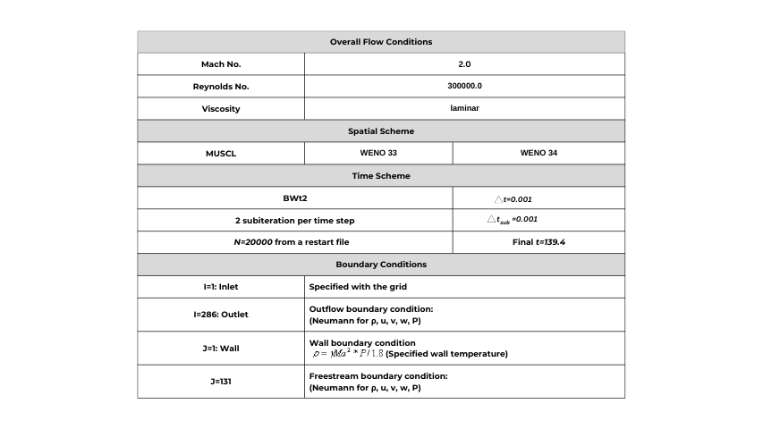
The problem simulates the complex separated flow field generated by the impingement of an oblique shock on a laminar boundary layer developed along a flat plate. The flow conditions are freestream Mach number of 2.0, shock flow deflection angle 6º, and Reynolds number ReL (based on the distance from the plate leading edge to the inviscid shock impingement location) equal to 3.0 ´ 105.

Mesh

The size of the 2D computational domain is 286 x 131. The mesh grid is shown in Figure 1.

Figure 2. Computational Mesh

Simulation Parameters

The simulation parameters are summarized in Table 1.The simulation parameters are summarized in Table 1.

Table 1. Simulation Parameters

Obtain the Files

Both mesh files and project input files can be accessed below. Remember to place the grid files in a subfolder with the set up file /shockbl.

Grid file

Start the Simulation

Change the directory to the subfolder with the selected grid and spatial scheme. Start the simulation by

mpirun –np 1 mpiaeroflo.exe < shockbl.afl

Simulation Results

Figures 2, 3 and 4 show the pressure contours of flow field for MUSCL, WENO 33 and WENO 34 procedures, respectively.

Comparison of Different Spatial Scheme

Figure 5 shows the surface pressure profiles for MUSCL and WENO procedures. The simulation results are also compared with Visbal and Gaitonde’s 3rd-order Roe scheme simulation using the same size mesh grid and a fine (476 x 265) mesh grid, respectively. WENO 34 scheme provide better results compared with MUSCL results.

CFL Test

The CFL performances for different spatial schemes are also tested for this problem. The test results are summarized in Table 2.

Table 2. CFL Number Test for Different Schemes

Reference

  1. Visbal, M. R. and Gaitonde, D. V., “Shock Capturing Using Compact-Differencing-Based Methods,” AIAA Paper 2005-1265.
  2. M. Visbal – private communication.

Table of Contents