The Shu-Osher problem simulates a normal shock front moving inside a one-dimensional inviscid flow with artificial density fluctuations. In the test case, the length of the computation domain is 1. The downstream flow is assumed to have a sinusoidal density fluctuation (ρ=1+εsin(x/λ)) with a wave length of λ = 1/8and an amplitude of ε = 0.2.A normal shock front with a Mach number of 3.0 is initially placed at the position x = λ. The initial conditions for the simulation are
ρ=3.857143; u=2.629369; P=10.3333 when x<1/8
ρ=1+0.2sin8x; u=0; P=1 when x≥1/8
Mesh
The mesh is an even spaced 1D grid. Two kinds of grids are used: a coarse grid (192 grid points) and a fine grid (384 grid points)
Simulation Parameters
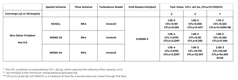
Table 1. Simulation Parameters for Shu-Osher Problem
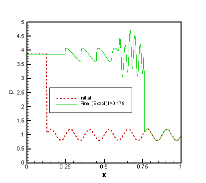
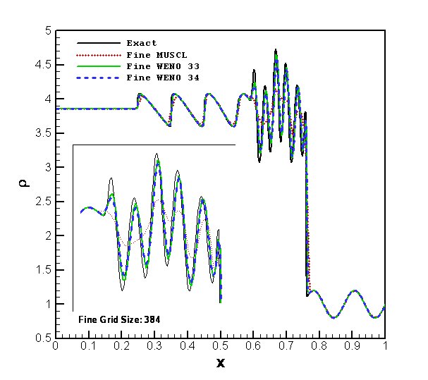
A WENO simulation result with a very fine grid (768 grid points) can be regarded as the exact solution. Figure 1 shows the initial density profile and the fine grid density profile at t = 0.178.
Table 1. Simulation Parameters for Shu-Osher Problem
Obtain the Files
Both mesh files and project input files can be accessed below. Remember to place the grid files in a subfolder with the set up file /shockwave.
Change the directory to the subfolder with the selected grid and spatial scheme. Start the simulation by
mpirun –np 1 mpiaeroflo.exe < shockwave.afl
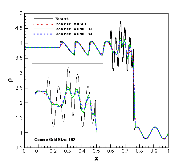
Comparison of Different Spatial Scheme
The MUSCL, WENO 33, and WENO 34 schemes are used for the simulations with a coarse grid (192 grid points) and a fine grid (384), respectively. The density profiles for different spatial schemes are shown in Figure 2 for coarse grid simulation and in Figure 3 for fine grid simulation, respectively. Both of the results are compared with the exact result. The result shows that the fine grid results are much better than coarse grid results and for the same grid simulation the WENO results (both 33 and 34 schemes) are better than MUSCL result, and WENO 34 is a little bit better than WENO 33.
Taylor, E.M., Wu, M., and Martin, M.P., “Optimization of Nonlinear Error for Weighted Essentially Non-Oscillatory Methods in Direct Numerical Simulations of Compressible Turbulence,” Journal of Computational Physics, Vol. 223, 2007, pp. 384-39