The duct test problem has been taken from Refs. [1-4]. Our predictions, in comparison with the experimental measurements, are shown in the next subsection. The agreement is excellent for the quantities compared. Details are presented below.
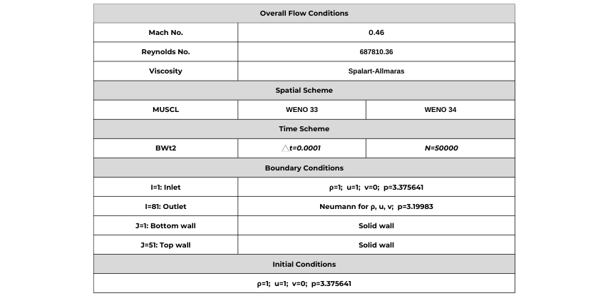
The physical domain has dimensions as shown in Fig. 1, where hthr = 0.14435 ft is used as the dimensional length scale. This provides a Mach number of 0.46 at inlet and a Reynolds number of 687,810.4.
Figure 1 Physical domain for converging-diverging duct calculation
The inlet total pressure and outlet pressures are 19.58 psi and 16.05 psi, respectively, with non-dimensional values of 3.37564 and 3.19983, respectively. The total temperature is 500oR. The density at the inlet is fixed at a non-dimensional value of 1.0. A non-dimensional velocity u = 1.0is applied at the inlet, while no-slip boundary conditions are imposed at the top and bottom walls. Dirichlet pressure boundary conditions are applied at the inlet and outlet, while zero Neumann boundary conditions are applied at the outlet for the other flow variables.
Mesh
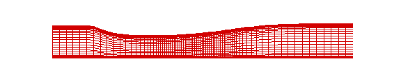
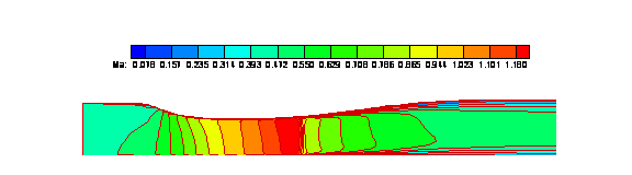
An 81 x 51 grid was used to calculate flow through the duct with grid clustering in the vicinity of solid walls. The mesh geometry is shown in Figure 2.
Figure 2. Computational Mesh
Simulation Parameters
Table 1. Simulation Parameters
Obtain the Files
Both mesh files and project input files can be accessed below. Remember to place the grid files in a subfolder with the set up file /cdvduct.
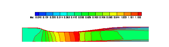
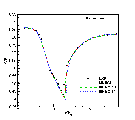
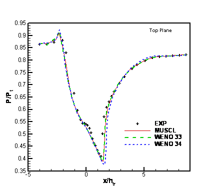
Figures 6 and 7 show the surface pressure distribution for different spatial schemes on the bottom wall and top walls, respectively. The results are also compared with experimental results.
Figure 8 compares the computation convergence speed for three spatial schemes.
Table 1. Simulation Parameters
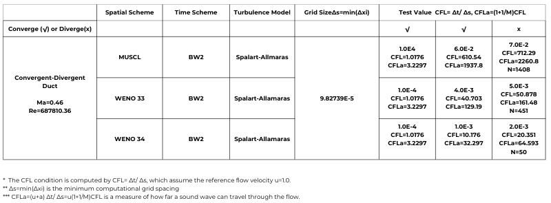
CFL Test
Table 1. Simulation Parameters
Reference
Bogar, T. J., Sajben, M., and Kroutil, J. C. (1983) “Characteristic Frequencies of Transonic Diffuser Flow Oscillations,” AIAA Journal, Vol. 21, No. 9, pp. 1232-1240.
Bogar, T. J. (1986) “Structure of Self-Excited Oscillations in Transonic Diffuser Flows,” AIAA Journal, Vol. 24, No. 1, pp. 54-61.
Chen, C. P., Sajben, M., and Kroutil, J. C. (1979) “Shock Wave Oscillations in a Transonic Diffuser Flow,” AIAA Journal, Vol. 17, No. 10, pp. 1076-1083.
Sajben, M., Bogar, T. J., and Kroutil, J. C. (1984) “Forced Oscillation Experiments in Supercritical Diffuser Flows,” AIAA Journal, Vol. 22, No. 4, pp. 465-474.
Salmon, J. T., Bogar, T. J., and Sajben, M. (1983) “Laser Doppler Velocimeter Measurements in Unsteady, Separated Transonic Diffuser Flows,” Vol. 21, No. 12, pp. 1690-1697.