Home > Sample Problems > Prandtl-Meyer Expansion
Prandtl-Meyer Expansion over a 15o
corner
at Mach =2.5
Problem
Statement
Analyze the supersonic flow expansion over a 15o corner at a Mach number M=2.5. The fluid is assumed to be an ideal gas with g=1.4, and the flow should be assumed inviscid. This type of flow is well known as the Prandtl-Meyer expansion and it has analytic solutions. The physical parameters and the computational grid for this test correspond to a NPARC Alliance Validation Archive test [1].
Governing
Equations
Since the flow is assumed inviscid, the Euler set of equations is solved.
Computational Grid
The computational grid is downloaded from the referenced website [1]. The format of the file is cgd (common grid file). This file is imported into ADF viewer. Using this software the x coordinates and the y coordinates are extracted into separate files, x.dat and y.dat, respectively. Following this step a small utility, CGDTOP3D.F90, is used to convert the two files into a single file, PM_exp.grd, containing the computational grid in PLOT3D format. The computational grid is shown in Fig. 1.
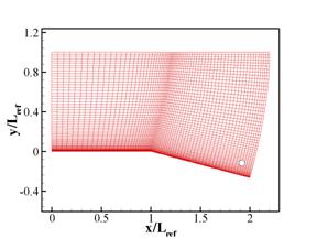
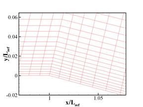
Fig. 1
Computational grid used for the simulation of supersonic expansion over a 15o corner at M=2.5.
The area around the corner marked with a rectangle in Fig. 1(a) is enlarged in
Fig. 1(b). The small circle in Fig. 1(a) marks the location (x,y)=(1.92,-0.12)
where the flow properties will be compared with analytical predictions.
Initial
Conditions
This problem will be analyzed as a transient one, using a uniform flow as initial condition. The density, velocity components, and pressure values are set to:
![]()
Boundary
Conditions
At i=1 (face=4), Dirichlet conditions are imposed for all variables. The values imposed are the same as the initial condition values above. At i=end, Neumann conditions are imposed since the flow remains supersonic throughout the field. At j=1, slip wall conditions are imposed. At j=end, Dirichlet conditions are imposed for all variables.
Spatial
Differentiation and Time Integration
The Beam-Warming algorithm was used to integrate the solution in time towards the steady-state. The computation time step was set to Dt = 5´10-3. Five sub-iterations were used for each time step. Both the MUSCL and the WENO scheme were used to compute the spatial differences. See the setup file in the appendix for specific parameters for the time and spatial schemes.
Turbulence
Model
For this case no turbulence model was used since the flow is inviscid.
Obtain the
Files
Setup file (pmexp.afl)
Grid file (pm_exp.grd).
Results
The temperature, pressure, and Mach number fields obtained from the numerical simulations are shown in Figs. 2 through 4, respectively. The results obtained with the MUSCL and the WENO schemes are qualitatively similar. Various flow properties sampled at (x,y) = (1.92, -0.12),which is a location where the supersonic expansion is completed, and are compared with analytical solutions in Table 1.
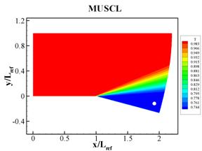

Fig. 2
Temperature fields corresponding to simulations using (a) MUSCL and (b) WENO
spatial difference schemes. The small circles mark the location where the flow
properties will be compared with analytical predictions.

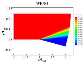
Fig. 3
Pressure fields corresponding to simulations using (a) MUSCL and (b) WENO
spatial difference schemes.
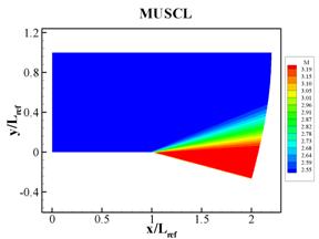

Fig. 4 Mach
number fields corresponding to simulations using (a) MUSCL and (b) WENO spatial
difference schemes.
|
|
Analytic |
AEROFLO-MUSCL |
AEROFLO-WENO |
| |||
|
Value |
%
Error |
Value |
%
Error |
Value |
%
Error | ||
|
M2 |
3.2368 |
3.2344 |
0.07 |
3.2349 |
0.06 |
3.04866 |
5.81 |
|
p2/p1 |
0.3274 |
0.327432 |
<0.01 |
0.32749 |
<0.01 |
0.32727 |
0.04 |
|
T2/T1 |
0.7269 |
0.727607 |
0.1 |
0.72748 |
0.08 |
0.77687 |
6.87 |
|
r2/r1 |
0.4505 |
0.450012 |
0.1 |
0.450175 |
0.07 |
0.42127 |
6.49 |
|
(p2/p1)0 |
1 |
0.99651 |
0.35 |
0.997297 |
0.27 |
0.75679 |
24.32 |
|
(T2/T1)0 |
1 |
0.9999805 |
<0.01 |
1.000015 |
<0.01 |
0.98709 |
1.29 |
Table 1. Comparison of flow properties at (x,y)=(1.92,-0.12)
obtained with AEROFLO using MUSCL and WENO schemes with analytical solutions and
previous results reported in Reference [1].
References
[1]
http://www.grc.nasa.gov/WWW/wind/valid/pm15/pm15.html
(cited on July 2, 2006)