Home   >  Sample Problems   >   Onera-M6-Wing (Multiblock)

 

Onera-M6-Wing

 

 

Problem Description

 

The transonic flow around the ONERA-M6-Wing was calculated using a multi-block grid. The pressure coefficient results for a Mach number of 0.8395 and an angle of attack of 3.06^o are compared with the experimental values of Schmitt and Charpin (1979).

 

Mesh

 

The number of grid points in each block is given in Table 1. The 3-block grid is a combination of two H-H grids (Blocks 1 and 2), for the upper and lower sides of the wing respectively, and a smaller C-type grid (Block 3) for a better solution near the leading edge of the wing. For Block 3, both a finer grid and a coarse grid are used.

 

Table 1. Number of grid points in the computational blocks

 

The topology of the computational mesh in Blocks 1 and 2 is presented in Figure 1. Although these two blocks are sufficient to compute the flow around the wing, a third block was also employed in order to improve the quality of the results near the leading edge of the wing. A detail of the Block 3 and its relative position with respect to the wing and Blocks 1 and 2 is shown in Figure 2. For Blocks 1 and 2a number of 50´33 grid lines are used on the wing surface.

 

 

 

 

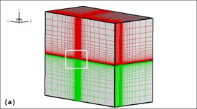
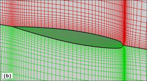
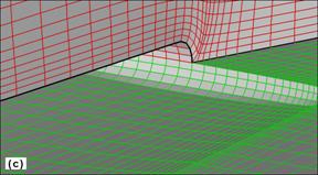
Figure 1. (a) Ensemble view of the H-H blocks around the Onera wing,

(b) detail near the wing surface at the symmetry plane, and (c) detail near the

wing tip with some of the planes from the upper block removed

to facilitate the view.

 

 

 

 

 

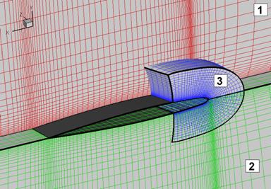
Figure 2. Computational grid around the wing. Some (x-y) planes from

Block 1 were blanked to enhance the view of the overlap with Block 3.

 

 

 

Simulation Parameters

 

 

Table 1. Simulation Parameters

 

The velocity components and density values were prescribed while the gradient of pressure was set to zero at i=i_max for Blocks 1 and 2. At the opposite boundary, i=1, as well as j=j_max, k=k_max for Block 1 and j=j_max, k=1 for Block 2, the velocity and density gradients were set to zero, while the pressure was imposed. At the interface between Blocks 1 and 2 (k=1 for Block 1, k=k_max for Block 2) the grid points are coupled except for 25 ≤ i ≤ 75, 1≤  j≤ 33 where slip wall conditions are imposed. For Block 3, slip wall conditions were imposed at k=1, while for k=k_max, i=1,i_max boundaries, the values are obtained from Blocks 1 and 2. For all blocks symmetry conditions were imposed at j=1.

 

The inviscid form of the compressible flow equations (also known as the Euler equations) was solved in the numerical simulations. Since viscosity is neglected, no turbulence model is necessary. The numerical simulations were performed using either the WENO (high-order) or MUSCL (low-order) scheme for spatial differencing and the Beam-Warming scheme for time advancement.

 

Obtain the Files

 

Both mesh files and project input files can be accessed below. Remember to place the grid files in a subfolder with the set up file /onera..

Setup file (onera_mb.afl)

Grid file (m6wing_v01_b1.grd, m6wing_v01_b2.grd, m6wing_v01_b3.grd, m6wing_v01_b5.grd).

 

Start the Simulation

 

Change the directory to the subfolder with the selected grid and spatial scheme. Start the simulation by

 

mpirun –np 3 mpiaeroflo.exe< onera.afl

 

The calculation starts from a previous MUSCL calculation which runs 15,000 steps from the initial calculation. The calculation will runs for another 10,000 steps to reach steady state.

 

Post Processing

 

A post processing tool postproc.exe can be found for both coarse and fine grid calculations. To extract the Tecplot format of wing surface pressure distribution file and span pressure coefficient distribution files, simply put the myres.dat and postproc.exe files in the same folder and run postproc.exe.

 

Simulation Results

 

Figures 4 and 5 are the MUSCL results of non-dimensionalized pressure contours on the top and bottom wing surfaces by using fine nose patch grid. Figures 6 and 7 are the WENO 33 results and Figures 8 and 9 are the WENO 34 results.

 

Figure 4. The Pressure Contour on Top Wing Surface for MUSCL Simulation with Fine Nose Patch

Figure 5. The Pressure Contour on Bottom Wing Surface for MUSCL Simulation with Fine Nose Patch

Figure 6. The Pressure Contour on Top Wing Surface for WENO 33 Simulation with Fine Nose Patch

Figure 7. The Pressure Contour on Bottom Wing Surface for WENO 33 Simulation with Fine Nose Patch

Figure 8. The Pressure Contour on Top Wing Surface for WENO 34 Simulation with Fine Nose Patch

Figure 9. The Pressure Contour on Bottom Wing Surface for WENO 34 Simulation with Fine Nose Patch

 

Comparison of Different Spatial Schemes

 

In order to determine the accuracy of the numerical results, the pressure coefficient at several wing span locations were compared to the experimental values. The results by using a coarse nose patch are shown in Figure 10, and the results by using a fine nose patch are shown in Figure 11.  It shows that both of the WENO calculations provide better results than MUSCL calculation.

 

Convergence Performance

 

The convergence is shown in Figure 12, which compares the iteration norm for the three spatial schemes.

Figure 10. Pressure coefficients at several wing span locations (coarse nose patch).

 

Figure 11. Pressure coefficients at several wing span locations (fine nose patch).

 

Figure 12 The Convergence of Three Spatial Schemes

 

 

Reference:

 

1. Schmitt, V. and Charpin, F., “Pressure Distributions on the Onera-M6-Wing at Transonic Mach Numbers,” Experimental Data Base for Computer Program Assessment. Report of the Fluid Dynamics Panel Working Group 04, AGARD AR 138, May 1979